Complete guide on logistic regression with gene expression data: the math
A complete guide on how to use logistic regression. This is the first part where I introduce the concept, the relationship with linear regression, and the math behind the algorithm. This tutorial will provide all the necessary details to understand in deep the algorithm.

This is the index of this tutorial so you can choose which part interest you more:
- Introduction to logistic regression
- Linear regression and logistic regression
- The mathematical basis of logistic regression
- Sigmoid function
- Odds ratio
- Logistic regression matrix notation
- Maximum Likelihood Estimation
- summary
- Other resources
- Bibliography
The previous tutorials on linear regression:
1. First part on the math: here
2. Second part on python implementation, algorithm evaluation: here
3. Third part about regularization: here
Introduction to logistic regression
In the previous tutorial, we introduced the concept of supervised learning (working with labeled data). We discussed regression, where your task is to calculate the value of a dependent variable (y) using independent variables (X). We are introducing now the concept of classification. Since approximately 70 % of problems are classification problems, knowing classification techniques is essential in data science. The classification technique is a supervised machine learning algorithm that captures the relationship between input variables and the target variable. In this case, the algorithm is trained to predict to which category (or class) a data point is belonging (of course, based on its features). As we discussed before a model is analyzing the features of the data set and it trying to mathematically express the dependence between inputs and outputs. the difference between regression and classification is that the first estimates a dependent variable that is continuous and unbounded while the second estimates a variable that is discrete and finite (which are called classes). For example, estimating the revenue of a bookshop is a regression problem (the output of the model is continuous). Instead, estimating the selling of which book category is bought is a classification problem. Logistic regression is a classification technique used to solve binary classification problems. It is one of the basic and older techniques, but it is still widely used. An extension of logistic regression is Multinomial or multiclass classification, used to solve a problem where you have to handle multiple classes in the target variable (y).
When can you use logistic regression? Here, are some examples:
- Spam detection.
- Customer purchase (if a customer would purchase or not a particular item if the customer would click on an advertisement).
- In the health domain: diabetes prediction, adverse event prediction, if a mass is benign or malign
- Credit card fraud
- Predict if a customer will default or not.
- Predict if an employee would be promoted
- Classify articles
Logistic regression has been extensively studied, it is one of the easiest algorithm to implement (especially for binary classification, where you have two classes). Generally, it is used as a baseline for classification problems.
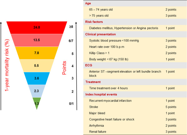
In oncology and cancer research, logistic regression has been used for risk stratification of patients (1). Risk stratification is an important tool in medicine to assign risk to a patient. Risk stratification is answering similar questions:
- Diagnosis: what is the likelihood of a patient having a particular disease?
- Prognosis: What is the survival probability of a patient after 5 years?
- Response to treatment: Is the patient responding well to treatment? Is the treatment effective?
- Disease prevention: is this screening required for the patient?
As you can see, most of these questions require a binary response. Demographics, symptoms, and other medical exam results are your features. Nowadays, genetic features are incorporated in risk models. One of the first models (1970) was the Framingham risk score to estimate if a patient was developing coronary heart disease. Since then, many risk scores have been developed (from breast cancer to other pathologies). A risk score that assesses the screening need, allows to focus on the high-risk patients and prevent the insurgence disease. Logistic regression has been widely used, but it has the drawback to assume a linear relationship (which is not the case with deep learning methods, so in specific cases these models are preferred). As we will discuss later in this tutorial, one advantage of logistic regression in risk stratification is its interpretability. Thus, the regression coefficient may be used to create a risk score for each individual and to evaluate the individual contribution of each feature to the output.
So, as we have seen before we have:
- Independent variables (or inputs, predictors, features, or X). If you have only one dependent variable is called x and it is a vector (from 1 to n), with more input variables you have a matrix.
- Dependent variable (or output, response, or y). if you have two classes this is a binary classification (the classes are generally indicated as 0 and 1, true and false, or positive and negative). If you have three or more classes as output you have a multiclass or multinomial classification. Another case is ordinal logistic regression where the target variable comprehends three or more ordinal categories (as an example product rating ranging from 1 to 5)
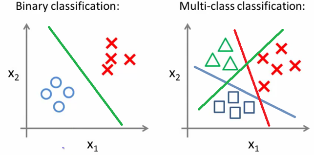
if we take a random dataset and we represent one variable (x1) and the y, we clearly see it is a binary classification problem.

Linear regression and logistic regression
Logistic regression is a statistical method for predicting binary classes (in other words the outcome is dichotomous). We can consider logistic regression as a special case of linear regression where the target variable is categorical and binary. In general, logistic regression predict the probabilities of occurrence of a binary event (the odds of one of the possible outcomes) through the logit function. In the next section, we will deepen this.
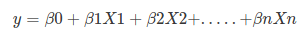
As we have seen in the previous tutorial, the equation of linear regression:
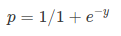
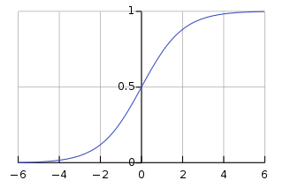
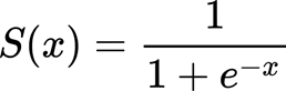
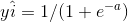
And this is the sigmoid function:
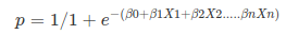
If we apply the sigmoid function on linear regression:
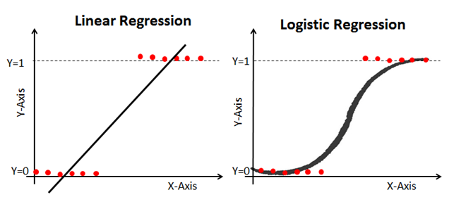
Linear regression as we have seen it is providing a continuous output, instead logistic regression is providing constant output. To find the best weight we use the Maximum Likelihood Estimation (MLE) approach when we train a logistic model. In the figure below, we can see that if we have a dependent variable that has only two categories (example: malignant or benign mass) it is clearly better to use logistic regression.
In summary, the difference and similarities between linear and logistic regression are:
- The output variable is continuous in linear regression (since real numbers, it can range from -∞ to +∞) while discrete and binary in logistic regression.
- Weight estimation in linear regression is conducted using Ordinary Least Squares (OLS) while you use Maximum Likelihood Estimation (MLE) in logistic regression.
- For the model fitness, you do not use R square (and other metrics) but you use a concordance, KS-statistics (and other metrics which will be discussed in detail below).
- The dependent variable in logistic regression follows the Bernoulli distribution while in linear regression target variable is a gaussian.
- As in linear regression, we assume no correlation (or multi-collinearity) between the independent variables
- Logistic regression is also sensible to the outliers.
if you want to know more about linear regression on genomic data:
The mathematical basis of logistic regression
We will discuss in detail in this section the basis of the logistic regression algorithm.
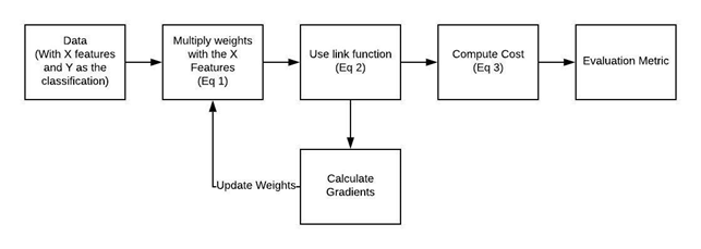
As we notice in the figure below, the flow of the algorithm is similar to linear regression. We have some weights associated with features used in a link function (the sigmoid in this case), we compute a cost function, we update the weights (using gradients) in the idea of minimizing the cost function, and then we have evaluation metrics.
We are now discussing some concepts that will be fundamental to understanding the algorithm.
Sigmoid function
Let’s start with the sigmoid function. A sigmoid is basically a mathematical function showing a characteristic S-shape (which is called a sigmoid curve).
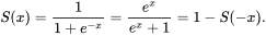
The logistic function is a sigmoid:
the logistic function is not the only sigmoid function existing, there are many more. Many of them have been used in neural networks as activation functions (tangent functions for example). In the figure below, you can see different sigmoid functions that are compared (all are normalized so the slope origin is 1).
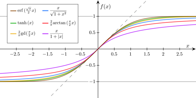
Interestingly, many natural processes exhibit a progression that is small at the beginning and it is accelerating until it reaches a climax. In chemistry, you observe a sigmoid curve in the titration between strong acid and bases. In biology, there are different examples in biochemistry.
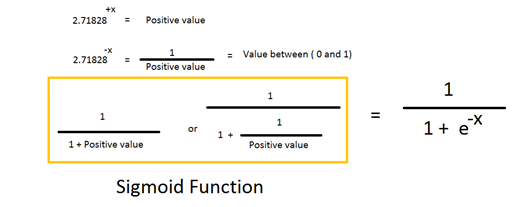
What is the little “e” in the function? It is the Euler’s number that is indicated with e, and it is often used in mathematics. You can calculate with this formula:
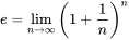
As n is approaching infinite the value is close to 2.71828
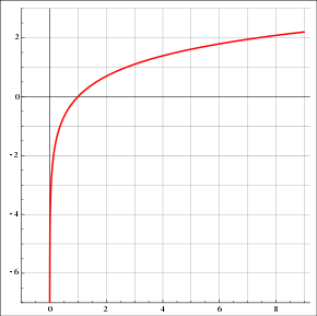
The natural exponent function:
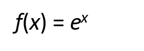
And in the figure the natural exponential function:
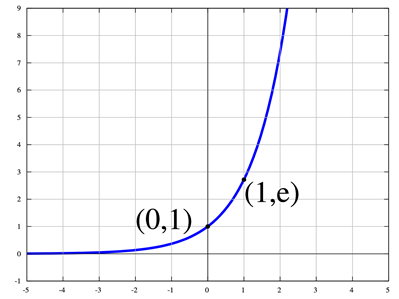
This function has different properties, one of the most known is that is derivative function is the same.
Why do we use the sigmoid function in logistic regression? Because it allows us to have values between 0 and 1.
Odds ratio
The odds ratio is the odds in favor of a particular event. It quantifies the strength of the association between two events. If A is the probability that a mass is malign and B the probability that mass is benign, then the odds are equal to A/B.
If we consider malign mass the event of interest, the odds ratio:
Odds ratio = P/(1-P)
The probability is ranging between 0 (no event) and 1. In general, you consider P the possibility of success (an event happening, admission in a university) and you define Q the failure.
Probability of success (P) = 0.8
Probability of failure (Q) = 1- P = 0.2
Odds are the ratio of the probability of success versus probability of failure, then:
Odds (Success) = P/Q = 0.8/0.2 = 4
Odds (Failure) = Q/P = 0.2/0.8 = 0.25
As a simple example, imagine we have two groups of patients, treated with the drug A or B. with the drug A on 10 patients, 7 survived. While with the drug B, on 10 patients, 3 survived. What is the probability of surviving for the patients treated with drug A?
P is the probability of surviving, while Q is the contrary. For drug A:
P = 7/10 = 0.7
Q = 1 — P = 1–0.7 = 0.3
While for the drug B.
P = 3/10 = 0.3
Q = 1 — P = 1–0.3 = 0.7
The odds of surviving:
Odd (A) = 0.7/0.3 = 2.33
Odd (B) = 0.3/0.7 = 0.42
The odds ratio is 2.33/0.42 = 5.44
As general formula then:
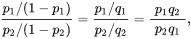
Logistic regression matrix notation
On this point, you can check this great tutorial: here.
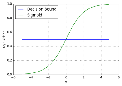
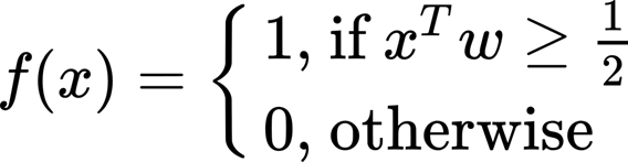
Logistic regression as said can also be considered as a linear regression special case where you have a binary classification problem (0 and 1). The problem can be described as a function that generates a predicted response that is close as possible to the actual response y, but the predicted has to be close to 0 or 1 since there are only two possible outputs. Considering the output of the function f(x) if the value is more than 0.5, the y is 1 (meaning the label is 1) otherwise is 0. 0.5 is the threshold or decision boundary, the value over that an observation is classified with another label.
In this case, the x is a vector (a feature vector), w is the associated weight and there is a bias (a constant we are not writing that is associated to the feature vector).
As we have seen in the previous tutorial on linear regression, this is the equation of linear regression.
The output of this formula is not giving any insight into a binary classification problem. The obtained output is ranging from -∞ to +∞, but we need something ranging from 0 and 1. So we need to combine this equation with something allowing us to have the desired output. For this, we are using the sigmoid function.
Which can also be rewritten as:
Remember that B0, B1, Bn are called estimators or regression coefficients (or also the weights).
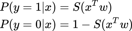
Why p? because we can interpret the output as probabilities. In concrete, the output of logistic regression is that input is belonging to a class labeled as 1. And as we have seen, before we can also calculate the probability that our input belongs to class 0. Y here is the true class label of our input x. the function f(x) or p(x) is often considered as the predicted probability that the output for a given x is equal to 1. Then for class 0, the predicted probability for a given x is 1- p(x).
As we have seen before in the linear regression tutorial, we do not know the weights. We have to find the value of this weight; the model learns this weight using the examples (data points with a ground truth label). The process of calculating the best weights using the available observations is called model training or fitting. We use the predicted output and we confront the ground-truth value to minimize the difference. The predicted y is also named y-hat. We have an X matrix with contains all the features for our dataset, w is a vector that comprises the weights for all the features, and by multiplying them we obtain the predictions. For a dataset, we obtain a y-hat as a vector containing the predicted labels. So, our sigmoid function can write like this:
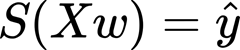
The idea is to combine this with the sigmoid curve and to isolate Xw.
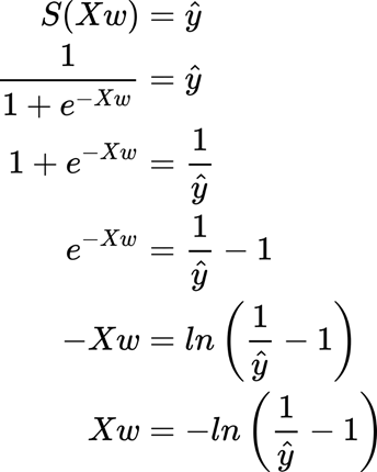
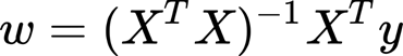
This is the closed-form to find the weights (using matrix calculation).
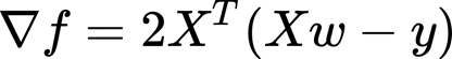
Instead, what we see here is the gradient (for more information on the gradient and stochastic gradient descendent (SGD) check the previous tutorial).
The formulas above are for linear regression. We can do the substitution:
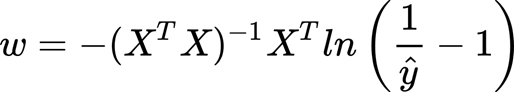
And the gradient:
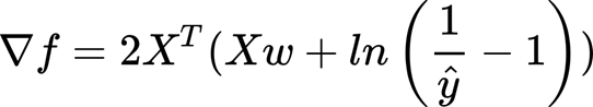
Can we use the sum of squared error (SSE) as a cost function?
Since the output is a probability SSE is not the best idea, it works great for linear regression but we need a better tool.
Maximum Likelihood Estimation
Maximum Likelihood Estimation (MLE) is a method for maximizing the likelihood, while the Ordinary least square method (the method used in linear regression) is for minimizing a distance. The idea is that by maximizing the likelihood function we determine the parameters (the weight) that are most likely producing the observed data (the labels for that datapoints). MLE sets the mean and variance needed for predicting data in a normal distribution.
OLS as we have seen is computed by fitting a regression line for the data points and calculating the distance with the real data (and on that is calculated the sum of the squared deviations). Since the output of logistic regression is a probability, MLE is a better method for this case.
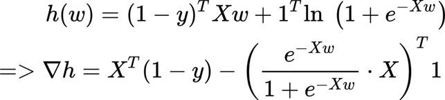
The equation of maximum likelihood estimation:
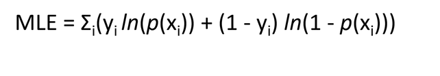
Ln is the natural logarithm. The natural logarithm function is a logarithm function with the logarithm base equivalent to e (Euler’s number). In other words, the natural logarithm of x is the power (or exponent) to which e would have to be raised to be equal to x. practically if x = 7.5
Ln(7.5) = 2.0149
Since e^2.0149 = 7.5
The image below shows the natural logarithm for some variable x for values comprised between 0 and 1. As the natural logarithm of x is coming close to zero is approaching negative infinity, while is 0 for ln(x) with x = 0. The opposite is true for ln(1-x). why there is a written log(x) instead of ln? in python (and it is true also for R language) in different libraries log(x) represents the natural logarithm of x. if you use NumPy log(x) it will calculate the natural logarithm of x.
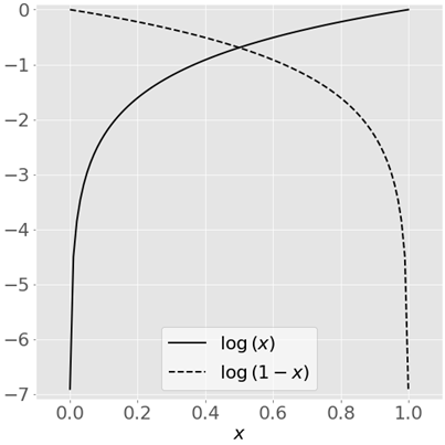
For a given x, when y= 0, then MLE is ln(1- p(xi)) and if p(xi) is close yi = 0 then the ln(1 — p(xi)) is close to 0. This is what we want if the actual value of y is 0, we want the y-hat to be 0 and we want that the probability is close to 0.
When y = 1, MLE for that observation (or data point) is yi*ln(p(xi)). If p(xi) is 1, then yi*ln(p(xi)) is 0, more p(xi) is approaching 1 more the logarithm is close to zero. And also, as we have seen in the image above, more p(xi) is far from 1, and more the logarithm is a large negative number. The idea is indeed to maximize the cost function (basically the closest to zero as possible) while large negative numbers are meaning a high error.
Now, we are describing this using the matrix notation. The likelihood function is the joint probabilities of the labels (the dependent variable) given the inputs (the independent variables, in fact, we are assuming the inputs are independents). Indeed, the likelihood can be written as the product of the probabilities of each data point (or observations). For a dataset of m observations:
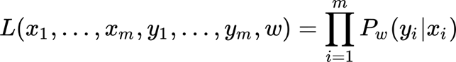
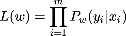
This function L is considering the weights but also the inputs (x) and the true labels (y), if we consider the last two as a constant that we cannot change we can rewrite the equation like this:
As we have seen above, we can rewrite the probabilities for each class label (where P is the probability for class 1, and then for class 0 is 1- P)
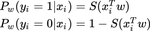
And in a compact form:

Which is in concrete the same of:
Ok starting from the likelihood function and using the matrix notation, we are interested in finding when this function is maximum (argmax).
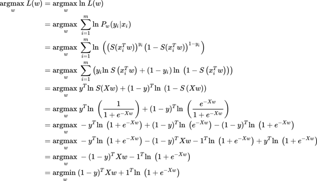
Finding a closed form is difficult, but we can use the gradient (and stochastic gradient descendant) to find the optimal weights.
One of the reasons we use likelihood as a cost function is that mean squared error is not finding the global minimum when applying to logistic regression (is not convex).
Summary
We have a matrix of inputs (x) with weight (w) and a dependent variable (y, with labels 0 and 1). The objective is to predict the class labels (y) for the observations (x). we do this by multiplying each feature (x) by the corresponding weight (w).

Transforming this with the sigmoid function:
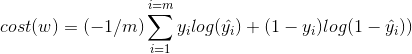
We then calculate the cost function:
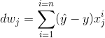
We calculate the derivative of the cost function or gradient:
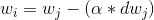
We multiply the derivative for a hyperparameter (alpha or learning rate) and we use that to update the weight.
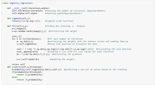
If we want to implement this in python from scratch:
if you have found it interesting:
Please share it, you can also subscribe to get notified when I publish articles, you can also connect or reach me on LinkedIn. Thanks for your support!
Here, is the link to my Github repository where I am planning to collect code, and many resources related to machine learning, artificial intelligence, and more.
Other resources
If you want to know more about the odds ratio: here
logistic regression math: here
on the natural logarithm: here
if you want to implement logistic regression from scratch: here
Bibliography
1. Imperiale TF, Monahan PO. Risk Stratification Strategies for Colorectal Cancer Screening: From Logistic Regression to Artificial Intelligence. Gastrointest Endosc Clin N Am (2020) 30:423–440. doi:10.1016/j.giec.2020.02.004
2. Cenko E, Ricci B, Bugiardini R. “STEMI: Prognosis,” in Encyclopedia of Cardiovascular Research and Medicine, eds. R. S. Vasan, D. B. Sawyer (Oxford: Elsevier), 489–498. doi:10.1016/B978–0–12–809657–4.99745-X